The scientific issues and historical developments outlined above led us to design the FIRST survey with the following specific goals:
In addition, uniformity of sensitivity over the full survey area and maximum achievable observing efficiency were important considerations, as were our ability to reduce and analyze the data in a timely fashion. We present here our solutions to the problems of sky coverage, efficiency and uniformity as well as other technical considerations involved in planning the survey, while the following section describes in detail how the observations are actually undertaken.
The goal of the survey is to produce a continuous, uniform-sensitivity 1.4 GHz image covering the north Galactic cap. The grid of pointing positions is chosen so that when the individual field maps are coadded (see § 6) the resulting images have nearly the same sensitivity at field centers as at the ``seams'' between the fields. As discussed by Condon et al. (1994), the optimal grid would be a simple hexagonal pattern if the sky were flat, but is more complicated on the celestial sphere. We designed the grid for the FIRST survey based on several requirements:
J. Condon originally proposed dividing the sky into declination strips
with each strip having a fixed RA and Dec spacing. This pattern is
inefficient for two reasons. First, since lines of constant RA
converge as they move away from the equator, the pointing centers are
more closely packed at the high-declination edge of each strip than at
the low-declination edge. To avoid wide variations in sensitivity it
is therefore necessary for the declination strips to be relatively
narrow (-
), and even these strips waste some
observing time near the high-declination edge because the centers are too
closely spaced. Second, it is necessary to observe the declination
line at the boundaries between strips twice (with two different RA
spacings) to avoid low-sensitivity holes in the coadded maps near the
boundary. This makes narrow strips inefficient.
The solution to these problems is to keep the RA spacing fixed
within strips but to allow the declination spacing to vary. At higher
declinations, where the constant RA lines have converged, the declination
spacing is correspondingly increased so that the sensitivity in
the coadded map remains constant. The declination spacing
required is roughly , which leads
to a constant number of pointing centers per unit area on the sphere; the
actual spacing we are using was computed so that the worst-case
sensitivity at any point in the coadded maps is the same everywhere
in the sky.
With variable declination spacing, the declination strips can be
much wider while still retaining high efficiency. A regular
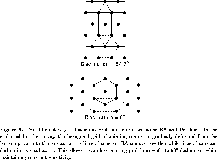
hexagonal grid
can be oriented along lines of RA and declination in two different
ways (see Fig. 3). If the distance between neighboring field
centers is , then the spacing along RA and declination lines is
in one direction and
in the other.
A natural way to lay out the declination strips is to start
with the grid oriented as in the lower panel of Figure 3 at the low-declination
edge and to allow the squeezing in RA and stretching in declination
to effect a gradual transformation of
the grid to the upper orientation in Figure 3.
This allows declination strips with
; for example,
a single declination strip can extend from
to
.
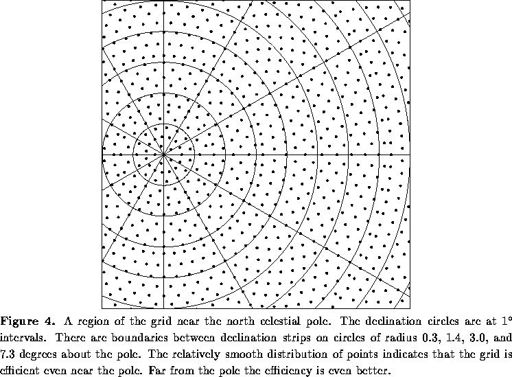
This scheme can be made even more efficient if we allow the declination
strips to be slightly wider, so that . Then the RA spacing (which jumps at strip boundaries) changes by
exactly a factor of 2 between strips. As a result, there is no need
for duplicate observations along the boundary declination; instead, as
one moves across the boundary, there is a seamless join between the 2
strips (Fig. 4). The resulting grid can be extended all the way to
the celestial pole with 7 declination strips.
The actual RA and declination values for the grid are described in
Tables 2 and 3.
The grid covers the sky over the
declination range to
. The positions lie on
lines of constant Right Ascension and Declination in J2000 coordinates.
The sky is divided up into 7 different declination zones. Within each
zone the number of RA points, NRA, is the same for all Dec rows.
A summary of the Dec zones is given in Table 2.
Table 3 gives the positions of the northern part of the survey grid.
The pointing centers on adjacent declination lines are staggered in
RA. For example, the Dec = line has RA =
,
, etc., while the next
line at Dec =
has RA =
,
, and so on. The RA values for row
are
,
,
where
if
is even and 1 if
is odd and
minutes.
At the boundaries of the declination zones, the number of RA points on each declination line changes by a factor of 2 (or by a factor of 3 for the dec zone at the pole.) As a result, as one crosses the zone boundary, every other RA point is dropped from the grid.
The rows are numbered such that row 0 is at the pole. The grid is
symmetrical about the equator, with row 356 on the equator, so the
declination of row is equal to minus the declination of row
. This symmetry makes it simple to extend the grid farther south
if desired. The number of fields covering the entire sky would be
265,452. For comparison, a ``perfect'' hexagonal grid with 26 arcmin
spacing covering a plane area of 41,253 square degrees would require
253,677 pointings, so the average efficiency of this grid over the sky
is 95.6%.
All declinations have been chosen to be integral multiples of 6 arcsec, and all RAs are integral multiples of 1.5 minutes of time. The positions can be specified exactly by giving the declination to an accuracy of 0.1 arcmin and the RA to 0.1 minute, allowing them to be coded in 11 characters: hhmmm+ddmmm.
As discussed above, the optimization of the grid pattern was an essential step in making efficient use of the VLA. Another measure of efficiency is the fraction of observing time actually utilized in collecting survey data. There are two primary sources of overhead in carrying out the observations: slewing and calibration. The stability of the VLA at 20cm allows calibration to be held to a minimum. In general, calibrators are observed once an hour for 60 s. Furthermore, calibration sources which lie close to the grid locations are selected in order to minimize slew time. Typically, less than 2 minutes per hour, or 3%of the observing time, is employed in calibration. As for time spent slewing between grid points, the VLA staff developed a special mode for observing equally spaced fields situated along lines of constant RA or declination. Using this survey mode, slew times between adjacent fields average 10 s, and account for a total of 6%of the allocated observing time. Another 3%of the time is lost to VLA down-time and periods of extreme interference. In summary, then, the FIRST survey uses 88%of its allocated hours integrating on target, a measure of efficiency which exceeds that of most normal observing programs at the Observatory despite our short integration time on each survey field.
The reduction of the accumulated data is computer intensive and was a major concern in evaluating the viability of the FIRST survey. We have subsequently demonstrated that the timely reduction and analysis of the observations is a tractable problem. We have divided the computations into three modules, each of which is accomplished through the use of an AIPS script of our design-one for editing and self-calibration, one for imaging and CLEANing, and one for coadding. Using a SPARC 10/40 processor, the scripts require 0.5, 1.5, and 0.5 hours, respectively, of real time per image processed. We currently have four such processors, adequate for reducing all the data taken in a given B configuration before the beginning of the subsequent observing season. Details of the pipeline processing system are contained in § 6.
In order to map the full primary beam of the VLA antennas () in
the B configuration, it is essential to perform the observations in the
bandwidth synthesis mode in order to avoid substantial bandwidth smearing. This
requirement has ancillary consequences. A major advantage is interference
suppression. Since narrow-band, man-made signals dominate the interference
environment most of the time, judicious selection of the center frequency of
each IF plus the editing of data on a channel by channel basis allows us to
operate at any time of day with a very small amount of time lost to
interference; in the 1993 data, fewer than 40 out of 2153 fields will require
reobservation owing to interference of any type. Our selected channel width
of 3 MHz leads to a limit on the reduction in peak intensity due to
bandwidth smearing of
at all points in the final coadded images.
The primary disadvantage to the bandwidth synthesis mode is the loss of half
the available bandwidth owing to correlator limitations, and the concomitant
loss of polarization information. Since the NVSS will achieve
polarimetric measurements for all sources brighter than mJy (for
a fractional polarization of 5%), and
fainter sources will nearly all have unmeasurably low polarized signals, this
is not a significant loss to the whole VLA sky survey program.