| Catalog Download Links | |
|---|---|
| Radio Text catalog: | table2_radio.txt.gz |
| Radio Text catalog (ApJ MRT): | apjsab0e89t2_mrt.txt.gz |
| Radio FITS catalog: | table2_radio.fits.gz |
| Radio Islands (segmentation) image: | m33-fixbeam-islands-2018aug31.fits.gz |
| Detection image: | m33-fixbeam-total-filter-2018aug31.fits |
| SNR Text catalog: | table4_snr_forced.txt.gz |
| SNR Text catalog (ApJ MRT): | apjsab0e89t4_mrt.txt.gz |
| SNR FITS catalog: | table4_snr_forced.fits.gz |
| SNR Islands image: | m33-snr-islands-2018aug31.fits.gz |
| X-ray Text catalog: | table6_xray_forced.txt.gz |
| X-ray Text catalog (ApJ MRT): | apjsab0e89t6_mrt.txt.gz |
| X-ray FITS catalog: | table6_xray_forced.fits.gz |
| X-ray Islands image: | m33-xray-islands-2018aug31.fits.gz |
This web page includes a description and links to data from the paper "A New, Deep JVLA Radio Survey of M33" by White, Long, Becker, Blair, Helfand & Winkler (2019, ApJS, 241, 37). See that paper for more details. See the M33 Home Page for a simple image browsing tool that shows radio and optical images along with catalogs and island (segmentation) boundaries. The M33 image cutout server provides an easy way to examine the radio, H-alpha, X-ray, etc. images at a particular position or at a list of positions.
The 1.4 GHz plus 5 GHz detection image was created by averaging the entire 5 GHz and 1.4 GHz bandpasses. The 1.4 GHz high and low frequency images were used, and 14 of the 16 125-MHz channels from the 5 GHz observations were used. (5 GHz channels 1 and 2 were contaminated by interference.) For the catalog data processing, the 5 GHz frequency channels were divided into two broad bands with the means of the 7 low-frequency channels and the 7 high-frequency channels. The 5 GHz and 1.4 GHz bands are equally weighted in the combined image. That is not optimal for a typical extragalactic source (which has a power law spectrum να with spectral index α=-0.7) but is a reasonably "spectrum-neutral" weighting for the source detection. The resulting source lists do not appear to be a strong function of the weighting.
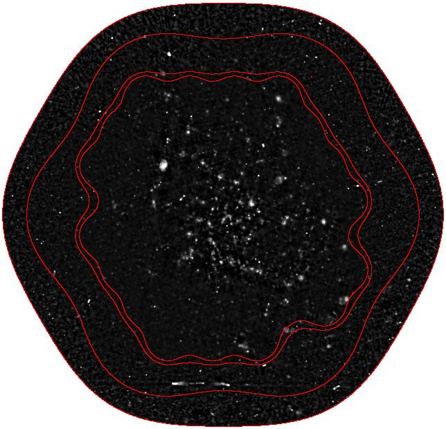
The sky coverage is not the same at all frequencies because the JVLA primary beam diameter is proportional to the observation frequency. The center of the field is covered by all four bands; the area covered by the low frequency 5 GHz is slightly larger; and the areas covered by the 1.4 GHz bands are much larger. The detection image is the average of the 1 to 4 available images. The figure to the right shows the detection image with the boundaries of the four frequency bands.
The images at all frequencies were convolved to a fixed round beam with FWHM 5.9 arcsec. That reduces the resolution of the final image, but it improves the consistency of the multi-resolution filtering step. It also produces much more accurate spectral indices when integrated over islands, where some fraction of the light might be spilling over the edges of the islands. This approach should produce more accurate flux densities and (especially) spectral indices than approaches that use the variable resolution images.
A multi-resolution (median pyramid) image processing algorithm was used both for source detection and to subtract the background from the image to make the source detection threshold more uniform. The images without background subtraction can be compared to the original summed image to see the effect of the background subtraction.
The island map (segmentation map) shows where sources where detected. The numbers in the island map correspond to the "Island" field in the catalog.
This catalog does not include Gaussian fits to the flux distribution within the islands. It simply integrates the fluxes within islands. This can dramatically increase the noise compared with Gaussian fits in some cases. For example, when a point source (FWHM = 5.9 arcsec) is embedded within a broad halo, an unweighted summation over the island adds a lot of noise from the extended halo region even if it does not contribute much to the flux. A Gaussian fit, in contrast, weights the pixels with flux much more heavily and effectively ignores the broad component. The result is much lower noise on the integrated flux density from the Gaussian.
However, the total flux determined from the Gaussian fits is likely to be quite inaccurate (and biased to be underestimated) compared with the island integrated fluxes. That is why we have decided not to include the Gaussian parameters. But to recover some of the benefits of flux weighting, we have created a fully multiresolution detection algorithm that divides the image up into a stack of images with varying resolution. The islands for a source are determined in each resolution channel, and the flux for that channel is integrated using only the pixels from the same channel. The effect is to use the noisiest, high-resolution structures only over small regions, and to use smoothed, lower-noise channels for low resolution structures. This reduces the noise in the integrated flux densities significantly while retaining a summation that adapts to any flux distribution within the image. For more details on this approach, see the paper.
The island boundaries at each resolution and frequency channel are determined using the FellWalker clump-finding algorithm. Islands detected at more than one resolution are merged. It is possible for several sources detected separately at high resolution to be embedded in one larger source at low resolution; in that case the morphology and sizes of the higher-resolution islands are used to determine how to break the large island into pieces. The FITS file with the island numbers is available for download above.
The integrated flux densities are computed over matching images for 4 frequency bands (splitting the 1.4 and 5 GHz bands in half). A PSF-dependent correction factor (close to unity) is applied to the sum of the flux within the island to correct for flux that spills outside the island. Sources in the outer region have fewer frequency bands measured; the nBands column tells how many bands were available for the source. The lowest nBands frequencies are always the ones that are available, with the higher frequencies missing.
Spectral indices are determined by fitting a power law to the band fluxes. The spectral index of the power law is constrained to be in the range -3 to 3. The flux density and error at a frequency of 1.4 GHz is given for convenience in comparing the results to other observations. But the most accurate flux model can be derived from the Fint column, which gives the power law normalization at the source-dependent pivot frequency pFreq. The pivot frequency is the frequency where the covariance between the spectral index and the flux normalization is zero, and it is also the frequency where the signal-to-noise (Fint/FiErr) is maximized. The flux density and uncertainty at other frequencies can be determined using propagation of errors from the FiErr and SpErr values.
The available bands are used to do the spectral index fit. The accuracy of the spectral index is much poorer when there are only 2 bands because of the reduced lever arm in frequency. No spectral index is given for sources with only a single band.
The moments in the island are used to determine the flux-weighted source position and major and minor axes (FWHM) of the equivalent elliptical Gaussian. Note that these sizes include the round 5.9 arcsec FWHM beam size. For an unresolved source the size will be approximately equal to 5.9 arcsec. The size is not constrained to be larger than this value; sources with sizes smaller than the beam PSF (due to noise fluctuations) will have integrated fluxes smaller than their peak fluxes.
The catalog also includes the peak flux density for the island computed from the detection image. The peak is simply the brightest pixel in the island. The RA_peak and Dec_peak columns give the position of the peak (which may not be the same as the flux-weighted mean position for asymmetrical sources). The position of the peak is determined in the sharpest channel of the median pyramid where the source is detected. That gives more accurate peak positions in crowded regions.
For the SNR and X-ray forced photometry catalogs, an island map is created using the size (and ellipticity, if available) of the external catalog. The island is padded to account for the 5.9 arcsec FWHM radio PSF. Then the radio flux density is integrated over the island. These catalogs are very similar in format to the radio catalog. The flux densities generally are noisier in these catalogs (even for detected sources) because they are not able to take advantage of multiresolution weighting to reduce noise in extended sources. The flux densities for externally specified islands are not adjusted to correct for radio emission that spills over the edges of the region.
The M33 radio catalog from the 5 GHz and 1.5 GHz data includes 2875 sources, 2868 of which are detected at 4-sigma or greater in the integrated flux density Fint. The catalog includes information about associated SNRs, H II regions and X-ray sources. Of the 7 sources that fall below the 4-sigma threshold, 6 are included because they have associated X-ray sources and 1 because it has an associated H II region; those faint objects are flagged in the Wrn column.
The catalog is available for download in text or FITS format. The text catalog has comments at the top that describe the contents. Here is a description of the columns in the text catalog:
| Radio catalog columns | ||
|---|---|---|
| Number | Column | Description |
| 1 | Name | Radio source name = W18-nnnn for island number nnn |
| 2 | RA | J2000 flux-weighted mean RA (hh:mm:ss.sss) |
| 3 | Dec | J2000 flux-weighted mean Declination (hh:mm:ss.sss) |
| 4 | RAPeak | (deg) RA (peak) |
| 5 | DecPeak | (deg) Declination (peak) |
| 6 | Wrn | W indicates source is below detection threshold |
| 7 | Ha-tot | (mW/m2) Integrated H-alpha flux |
| 8 | Ha-ave | (mW/m2/arcsec2) H-alpha surface brightness |
| 9 | F1.4GHz | (uJy) Flux at frequency 1.4 GHz |
| 10 | F1.4Err | (uJy) Error on F1.4GHz |
| 11 | Spind | Spectral index, Fnu = Fint*(nu/nu0)**Spind |
| 12 | SpErr | Error on SpErr |
| 13 | Fint | (uJy) Flux density at pivot frequency pFreq |
| 14 | FiErr | (uJy) Error on Fint |
| 15 | pFreq | (GHz) Pivot frequency where SNR is maximum |
| 16 | Fpeak | (uJy) Peak pixel in island |
| 17 | FpErr | (uJy) Noise in Isl_Fp |
| 18 | Major | (arcsec) Major axis FWHM (fitted, includes Gaussian beam with FWHM = 5.9 arcsec) |
| 19 | Minor | (arcsec) Minor axis FWHM (fitted, includes Gaussian beam with FWHM = 5.9 arcsec) |
| 20 | PA | (deg) Position angle of major axis |
| 21 | nBands | Number of frequency bands with data (1 to 4 of 1.3775, 1.8135, 4.679, 5.575 GHz) |
| 22 | Island | Island number (integer) |
| 23 | Sflag | SNR detection flag |
| 24 | SNRname1 | Name of associated SNR(s) |
| 25 | SNRname2 | Name of associated SNR(s) |
| 26 | SNRname3 | Name of associated SNR(s) |
| 27 | nXray | Number of associated X-ray sources |
| 28 | nHII | Number of associated H II regions |
The flag columns are intended to help make sense of cases with multiple matches (which are fairly common in this very crowded field). Multiple matches are listed in order of decreasing island overlap, so when the first match is considered most likely to be correct. The detection flags (Sflag in the table above, Rflag in the other tables) are bit flags where the bits are described below.
| Flag columns | |
|---|---|
| Value | Meaning |
| 1 | This source has at least one match in the external catalog. |
| 2 | Unambiguous match: this source matches only one object from external catalog. |
| 8 | Mutually good match (this source best for the other object, the other object is best for the source). |
These values are combined when a match satisfies more than one criterion. The most reliable matches will have flag bit 8 set. All of those will have bit 1 set as well, and most of them will also have bit 2 set. So the best matches have flag = 11, and most of the flag = 9 matches are also reliable. Flag values smaller than 9 indicate confusion about the best match, so the association should be treated with caution.
Here is the distribution of the Sflag values in the radio catalog:
| Flag Distribution in Radio Catalog | |||
|---|---|---|---|
| Value | Sflag | ||
| 0 | 2728 | ||
| 1 | 0 | ||
| 3 | 18 | ||
| 9 | 17 | ||
| 11 | 112 | ||
For many purposes we can choose samples that are not confused by excluding objects that have flag values other than 0, 9 or 11.
The forced photometry catalogs (for SNRs and X-ray sources) have similar columns. Additional fields are added giving information about the radio catalog and information from observations of the SNR in Long+ 2010 or Lee & Lee 2014. Here is the description for the SNR forced photometry catalog:
| SNR forced photometry catalog columns | ||
|---|---|---|
| Number | Column | Description |
| 1 | Source-name | Name of SNR from Long+ 2010 or Lee & Lee 2014 |
| 2 | RA | J2000 flux-weighted mean RA (hh:mm:ss.sss) |
| 3 | Dec | J2000 flux-weighted mean Declination (hh:mm:ss.sss) |
| 4 | R | (kpc) Galactocentric distance |
| 5 | D | (pc) SNR diameter |
| 6 | Opt | yes means SNR has SII/H-alpha > 0.4 |
| 7 | Xray | yes means SNR has XMM or Chandra X-ray detection |
| 8 | Radio | yes means radio flux is greater than 3 sigma |
| 9 | F1.4GHz | (uJy) Flux at frequency 1.4 GHz |
| 10 | F1.4Err | (uJy) Error on F1.4GHz |
| 11 | Spind | Spectral index, Fnu = Fint*(nu/nu0)**Spind |
| 12 | SpErr | Error on SpErr |
| 13 | Fint | (uJy) Flux density at pivot frequency pFreq |
| 14 | FiErr | (uJy) Error on Fint |
| 15 | pFreq | (GHz) Pivot frequency where SNR is maximum |
| 16 | nBands | Number of frequency bands with data (1 to 4 of 1.3775, 1.8135, 4.679, 5.575 GHz) |
| 17 | Rflag | Radio detection flag |
| 18 | RadName1 | Name of associated radio source(s) |
| 19 | RadName2 | Name of associated radio source(s) |
| 20 | RadName3 | Name of associated radio source(s) |
Here is the description for the X-ray forced photometry catalog:
| X-ray forced photometry catalog columns | ||
|---|---|---|
| Number | Column | Description |
| 1 | Source-name | Name of Chandra X-ray sources from ChASeM33 (Tuellmann+ 2011) |
| 2 | RA | J2000 flux-weighted mean RA (hh:mm:ss.sss) |
| 3 | Dec | J2000 flux-weighted mean Declination (hh:mm:ss.sss) |
| 4 | D | (pc) X-ray diameter |
| 5 | Counts-tot | total Chandra count rate |
| 6 | Counts-soft | Chandra count rate in soft band (0.35-1.0 keV) |
| 7 | Counts-med | Chandra count rate in medium band (1.0-2.0 keV) |
| 8 | Counts-hard | Chandra count rate in hard band (2.0-8.0 keV) |
| 9 | SNR | yes means source is associated with SNR |
| 10 | Radio | yes means radio flux is greater than 3 sigma |
| 11 | Ha-tot | (mW/m2) Integrated H-alpha flux |
| 12 | Ha-ave | (mW/m2/arcsec2) H-alpha surface brightness |
| 13 | F1.4GHz | (uJy) Flux at frequency 1.4 GHz |
| 14 | F1.4Err | (uJy) Error on F1.4GHz |
| 15 | Spind | Spectral index, Fnu = Fint*(nu/nu0)**Spind |
| 16 | SpErr | Error on SpErr |
| 17 | Fint | (uJy) Flux density at pivot frequency pFreq |
| 18 | FiErr | (uJy) Error on Fint |
| 19 | pFreq | (GHz) Pivot frequency where SNR is maximum |
| 20 | nBands | Number of frequency bands with data (1 to 4 of 1.3775, 1.8135, 4.679, 5.575 GHz) |
| 21 | Rflag | Radio detection flag |
| 22 | RadName1 | Name of associated radio source(s) |
| 23 | RadName2 | Name of associated radio source(s) |
| 24 | RadName3 | Name of associated radio source(s) |