The correlation function fit parameters for various subsamples are given in Table 1.
Sample          Source Type     Source Number   Amplitude (1E-3)  Power (gamma)
------          -----------     ------------    ----------------  -------------
all sources     mixed             109,873         3.7 +/- 0.3     -1.06 +/- 0.03
double+multi    FR I & II          17,773         3.8 +/- 0.5*    -1.39 +/- 0.4
single          UFR, SB & C        92,057         5.2 +/- 0.4     -0.84 +/- 0.05
single, S>3mJy  UFR, C & SB        33,800         1.9 +/- 0.4     -1.10 +/- 0.07
single, S<2mJy  SB, UFR & C        45,312         8.2 +/- 1.0     -0.84 +/- 0.05
all X Abell     mixed X clusters  109,873 X 382  13.5 +/- 4.8     -1.07 +/- 0.2
Fitted parameters for various subsamples of data. Values are obtained from the (DD/DR-1) method of estimation. Fitting is done out to 2\r{} except for the one labled with *, which is fitted to 0.2\r{}. C refers to `compact' sources, SB refers to starburst galaxies and FR refers to the Fanaroff-Riley classification. U stands for unresolved.
A catalog of 109,873 sources was generated by collapsing all sources that are
within ![]() of each other to a single source, since the majority
of such cases represent multiple components of a single host object (e.g.,
double radio lobes). This sample predominantly contains
radio-loud, giant elliptical galaxies, quasars, and
starbursting galaxies (Windhorst et al. 1985).
(Becker et al. (1996) have shown that stars make up less than
0.1% of the sources.)
The correlation function of such
a mixed sample is difficult to interpret but it serves as a starting point
for investigating specific subsamples. The correlation
function for all sources in the catalog with
of each other to a single source, since the majority
of such cases represent multiple components of a single host object (e.g.,
double radio lobes). This sample predominantly contains
radio-loud, giant elliptical galaxies, quasars, and
starbursting galaxies (Windhorst et al. 1985).
(Becker et al. (1996) have shown that stars make up less than
0.1% of the sources.)
The correlation function of such
a mixed sample is difficult to interpret but it serves as a starting point
for investigating specific subsamples. The correlation
function for all sources in the catalog with ![]() and
and
![]() was determined using both the LS estimator
[
was determined using both the LS estimator
[![]() ] and the S estimator
[
] and the S estimator
[![]() ]. The RR and DR used are the average of 10 random
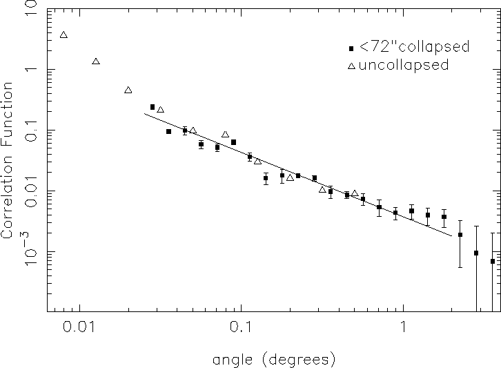
field generations. The results for the S estimate are displayed in
Figure 1.
The error bars shown are random errors determined using the bootstrap
algorithm described above.
]. The RR and DR used are the average of 10 random
field generations. The results for the S estimate are displayed in
Figure 1.
The error bars shown are random errors determined using the bootstrap
algorithm described above.

Figure 1:
The squares show the autocorrelation function (![]() )
calculated for the
whole sample (109,873 sources, where sources separated by less than
)
calculated for the
whole sample (109,873 sources, where sources separated by less than
![]() have been collapsed to a single source). The triangles show
the correlation function obtained when sources are not collapsed.
Error bars are
obtained using the bootstrapping technique described in Section 3.
have been collapsed to a single source). The triangles show
the correlation function obtained when sources are not collapsed.
Error bars are
obtained using the bootstrapping technique described in Section 3.
To determine the parameters of a power-law fit of the form ![]() ,
a straight line was fitted to the log-log plots (for collapsed sources)
out to
,
a straight line was fitted to the log-log plots (for collapsed sources)
out to ![]() using
standard
using
standard ![]() minimization. This yields
minimization. This yields
![]() and
and ![]() for the S estimator and
for the S estimator and
![]() and
and ![]() for the LS estimator.
For the LS estimate to be a better
estimate than the S estimate, one requires many more random points in a field
than data points. With about
for the LS estimator.
For the LS estimate to be a better
estimate than the S estimate, one requires many more random points in a field
than data points. With about ![]() data points, the number of random points
is severely limited by computer time. The S estimate is thus
probably more reliable.
data points, the number of random points
is severely limited by computer time. The S estimate is thus
probably more reliable.
Also shown in Figure 1 are correlation function estimates obtained when
sources separated by less then ![]() are not collapsed. As is
expected, one sees a large increase in the correlation function on small
scales resulting from single sources being counted as two or more sources.
On the scales of our fit, however there is little difference between the
two, indicating that the small percentage of unassociated sources which
have been merged do not affect the correlation function significantly.
are not collapsed. As is
expected, one sees a large increase in the correlation function on small
scales resulting from single sources being counted as two or more sources.
On the scales of our fit, however there is little difference between the
two, indicating that the small percentage of unassociated sources which
have been merged do not affect the correlation function significantly.
There are two problems with fitting a straight line to
determine power law parameters. The first is that normal errors in the
original data do not translate to normal errors in the log-log plot as
required for ![]() fitting. To check
the effects of this, we used the Levenberg-Marquardt technique to fit
a function of the form
fitting. To check
the effects of this, we used the Levenberg-Marquardt technique to fit
a function of the form ![]() to the original (linear-linear)
data. It was found
that the slopes and amplitudes agreed to well within
to the original (linear-linear)
data. It was found
that the slopes and amplitudes agreed to well within ![]() with the
straight-line fits; we thus consider the straight-line fits to be adequate.
The second problem is that the correlation function estimates at different
with the
straight-line fits; we thus consider the straight-line fits to be adequate.
The second problem is that the correlation function estimates at different
![]() are not independent. In calculating the correlation function for
a sample of optical galaxies, Bernstein (1994) used principal component
analysis to obtain linearly independent combinations of their measurements
which could then be used in a
are not independent. In calculating the correlation function for
a sample of optical galaxies, Bernstein (1994) used principal component
analysis to obtain linearly independent combinations of their measurements
which could then be used in a ![]() fit. It did not appear to affect
their estimates of the parameters significantly (although the effect
on error estimates can be more substantial).
fit. It did not appear to affect
their estimates of the parameters significantly (although the effect
on error estimates can be more substantial).
As a test of our procedures, random fields were generated and
analyzed as though they were data fields. It was found that the ![]() were consistent with zero.
were consistent with zero.
Some systematic differences in the uniformity of the survey are evident in the
correlation functions. The result for the sample that
includes the sources flagged as sidelobes (not plotted) shows a sudden
increase in
![]() at
at ![]() . When flagged sources are removed (as in the
figures shown here),
the bump decreases in size but is still noticeable, particularly in the
result for
double and multi-component sources. Six arcminutes is the distance of the
first sidelobe in uncleaned VLA B-configuration images so the `bump' is a
clear indicator that not all
sidelobes have been removed. The situation is worse for double and
multi-component sources because the sidelobes from such extended sources
are harder to remove in the
standard cleaning process.
To investigate further the effect of sidelobes on the correlation function,
varying fractions of spurious sources were added at
. When flagged sources are removed (as in the
figures shown here),
the bump decreases in size but is still noticeable, particularly in the
result for
double and multi-component sources. Six arcminutes is the distance of the
first sidelobe in uncleaned VLA B-configuration images so the `bump' is a
clear indicator that not all
sidelobes have been removed. The situation is worse for double and
multi-component sources because the sidelobes from such extended sources
are harder to remove in the
standard cleaning process.
To investigate further the effect of sidelobes on the correlation function,
varying fractions of spurious sources were added at
![]() from real data points. Results indicate that the distortion
in the correlation function is fairly well
localised to
from real data points. Results indicate that the distortion
in the correlation function is fairly well
localised to ![]() and that about
and that about ![]() of all the
(collapsed) sources remaining in the catalog are sidelobes. Efforts to
improve the efficiency of our sidelobe flagging algorithms are in progress.
of all the
(collapsed) sources remaining in the catalog are sidelobes. Efforts to
improve the efficiency of our sidelobe flagging algorithms are in progress.
The first point in the correlation function for the
whole sample appears high. This could be attributed
to the presence of double-lobed galaxies that have separations larger
than ![]() , the adopted radius within which we call all detected
components a single radio source.
There is also a significant dip in
, the adopted radius within which we call all detected
components a single radio source.
There is also a significant dip in ![]() at
at ![]() . This
could be related to the cleaning procedure or to the systematic
non-uniformity in sensitivity that is repeated from one coadded map to
another. To
investigate this further we included the sensitivity fluctuations
given in the coverage map in the random field (as described in
. This
could be related to the cleaning procedure or to the systematic
non-uniformity in sensitivity that is repeated from one coadded map to
another. To
investigate this further we included the sensitivity fluctuations
given in the coverage map in the random field (as described in ![]() ). This
did result in a smoother estimate at
). This
did result in a smoother estimate at ![]() ; in addition, the first
point in the
correlation function was also slightly lower. Fitting a straight line
to the log-log data which included the sensitivity fluctuations returned
parameters which were within
; in addition, the first
point in the
correlation function was also slightly lower. Fitting a straight line
to the log-log data which included the sensitivity fluctuations returned
parameters which were within ![]() of those which did not include
sensitivity fluctuations (given above).
of those which did not include
sensitivity fluctuations (given above).
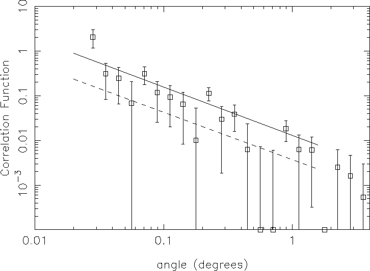
Cross-correlating the whole sample with Abell clusters results in a
power law fit with an amplitude ![]() times that of the
autocorrelation (see Figure 2). In the future, we will investigate the
possibility
of combining this information with spatial information for clusters to
infer spatial information for radio sources.
times that of the
autocorrelation (see Figure 2). In the future, we will investigate the
possibility
of combining this information with spatial information for clusters to
infer spatial information for radio sources.

Figure 2:
The cross-correlation function of the whole sample of radio sources
with Abell clusters using the Dd/Rd-1 estimator. The solid line shows the
best fit to the cross-correlation results while the dotted line shows the
best fit to the auto-correlation of the radio sources (S) estimator. Error
bars show Poissonian errors (![]() )
)
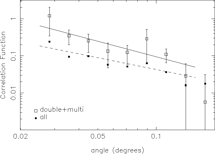
A catalog of double and multi-component sources (resolved extended sources)
was generated by considering
any sources separated by less than ![]() to be part of a single
multi-component source. Results for this subsample of 17,773 sources
using the S estimator are shown for
to be part of a single
multi-component source. Results for this subsample of 17,773 sources
using the S estimator are shown for ![]() in Fig. 3.
Force-fitting a line with the same slope as the whole sample
yields an amplitude of
in Fig. 3.
Force-fitting a line with the same slope as the whole sample
yields an amplitude of ![]() , a factor of 2.7 times larger
than that for the sample as a whole. Fitting a straight line on these small
scales
yields
, a factor of 2.7 times larger
than that for the sample as a whole. Fitting a straight line on these small
scales
yields ![]() and
and ![]() . On larger
scales many of the error bars extend below zero so we fit the linear-linear
data using the Levenberg-Marquardt technique. This yields
. On larger
scales many of the error bars extend below zero so we fit the linear-linear
data using the Levenberg-Marquardt technique. This yields
![]() and
and ![]() out to
out to ![]() , but this does not
fit the points on small scales very well.
, but this does not
fit the points on small scales very well.

Figure 3:
Open squares show the autocorrelation function for the double
and multi-component systems using the S estimator with the
solid line showing the best fit to the points. The filled squares and dashed
line are the same as those shown in Figure 1.
Traditionally, those radio sources which can be resolved into components have
been classified into one of two groups (Fanaroff and Riley 1974):
FR II sources are the more luminous
(![]() )
`classical doubles', while FR I sources have distorted lobe structures and
generally have lower luminosities. FR II sources are known to prefer lower
density environments than FR I sources at low z, but Hill and Lilly (1991)
have shown that at z
)
`classical doubles', while FR I sources have distorted lobe structures and
generally have lower luminosities. FR II sources are known to prefer lower
density environments than FR I sources at low z, but Hill and Lilly (1991)
have shown that at z![]() 0.5 FR II sources also exist in higher density
regions. In an attempt to estimate the correlation for
FR II and FR I sources separately, the catalog of multiple sources was split
into a catalog containing double sources only, and a catalog containing
sources with more than two components.
The small number of points resulted in a large amount of scatter, particularly
on larger scales, but on small scales (
0.5 FR II sources also exist in higher density
regions. In an attempt to estimate the correlation for
FR II and FR I sources separately, the catalog of multiple sources was split
into a catalog containing double sources only, and a catalog containing
sources with more than two components.
The small number of points resulted in a large amount of scatter, particularly
on larger scales, but on small scales (![]() ), it
appeared that the multi-component sources (predominantly FR I's)
were, as expected, more clustered than the double sources (FR II's) by
about a factor of 2-3.
), it
appeared that the multi-component sources (predominantly FR I's)
were, as expected, more clustered than the double sources (FR II's) by
about a factor of 2-3.
Using the preliminary catalog of sources with ![]() that was
available at the beginning of 1995, a catalog of double sources was
generated using stricter selection criteria than those used here. In addition
to the
requirement that there be two (and only two) sources separated by less than
that was
available at the beginning of 1995, a catalog of double sources was
generated using stricter selection criteria than those used here. In addition
to the
requirement that there be two (and only two) sources separated by less than
![]() , the fluxes of the sources were required to be within a
factor of five of each other. The correlation
function determined using the more limited sample agrees well with the
correlation function determined for the sample with the simpler
selection criteria.
, the fluxes of the sources were required to be within a
factor of five of each other. The correlation
function determined using the more limited sample agrees well with the
correlation function determined for the sample with the simpler
selection criteria.
The cross correlation of Abell clusters with double and multi-component
sources was determined. The correlation amplitude is a factor
of ![]() larger than that obtained for the cross-correlation with the
whole sample and
larger than that obtained for the cross-correlation with the
whole sample and ![]() larger than that obtained for the
autocorrelation of this subsample.
larger than that obtained for the
autocorrelation of this subsample.
We have also analyzed a sample that excluded all double and multi-component
sources. Fitting a straight line, one obtains ![]() and
and ![]() using the S estimate and
using the S estimate and
![]() and
and ![]() using the LS estimate. These slopes are
shallower than those
obtained for the sample as a whole, and are more consistent with values
determined from optical surveys. The difference is statistically not very
significant but it could be related to the fact that this
subsample contains a larger fraction of
starbursting galaxies as compared to the sample as a whole.
Bright, low-redshift starbusting galaxies are an important component of
extragalactic
IRAS sources which have been shown to have spatial clustering
properties similar to those found for optical galaxies (Davis et al. 1988).
The relative contributions of starburst galaxies and AGN to the cumulative
radio source counts is given in BWH as a function of flux density (based on
Windhorst et al. (1985) and Condon (1984)). Below 1.0 mJy
the ratio of the number of starbursting galaxies to the number of AGN
(including all giant ellipticals) is approaching unity. Above 3 mJy this
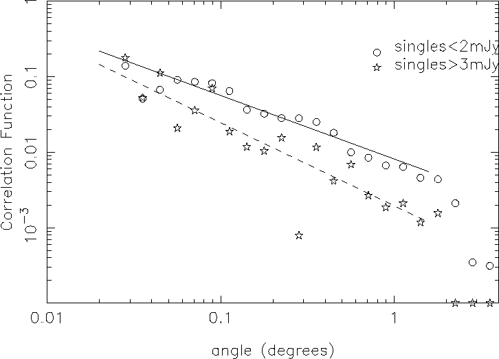
ratio becomes orders of magnitude smaller. To investigate the
contribution of starbursting galaxies to the correlation function, the
`singles' catalog was divided into catalogs of sources with flux densities
below 2 mJy and above 3 mJy, respectively. The results are shown in
Fig. 4.
Best fit parameters
to the S<2 mJy sources are
using the LS estimate. These slopes are
shallower than those
obtained for the sample as a whole, and are more consistent with values
determined from optical surveys. The difference is statistically not very
significant but it could be related to the fact that this
subsample contains a larger fraction of
starbursting galaxies as compared to the sample as a whole.
Bright, low-redshift starbusting galaxies are an important component of
extragalactic
IRAS sources which have been shown to have spatial clustering
properties similar to those found for optical galaxies (Davis et al. 1988).
The relative contributions of starburst galaxies and AGN to the cumulative
radio source counts is given in BWH as a function of flux density (based on
Windhorst et al. (1985) and Condon (1984)). Below 1.0 mJy
the ratio of the number of starbursting galaxies to the number of AGN
(including all giant ellipticals) is approaching unity. Above 3 mJy this
ratio becomes orders of magnitude smaller. To investigate the
contribution of starbursting galaxies to the correlation function, the
`singles' catalog was divided into catalogs of sources with flux densities
below 2 mJy and above 3 mJy, respectively. The results are shown in
Fig. 4.
Best fit parameters
to the S<2 mJy sources are ![]() and
and
![]() using the S estimator and
using the S estimator and ![]() and
and
![]() using the LS estimator. A similar result is obtained for
a sample with 2 mJy<S<3 mJy, indicating that incompleteness is not
a problem here. The shallow slope and large
amplitude is consistent with there being a larger contribution from `nearby'
starbursting galaxies with clustering properties more similar to optical
galaxies.
Best fit parameters
to the S>3 mJy sample are
using the LS estimator. A similar result is obtained for
a sample with 2 mJy<S<3 mJy, indicating that incompleteness is not
a problem here. The shallow slope and large
amplitude is consistent with there being a larger contribution from `nearby'
starbursting galaxies with clustering properties more similar to optical
galaxies.
Best fit parameters
to the S>3 mJy sample are ![]() and
and
![]() using the S estimator and
using the S estimator and ![]() and
and ![]() using the LS estimator.
Above 3 mJy the slope is more similar to that obtained
for all sources, but the amplitude is significantly
lower. Assuming that clustering does not decrease with
time, the clustering amplitude of a sample must decrease as the average
distance to the sources increases. The results are thus consistent with the
S> 3mJy sources being dominated by more distant, unresolved FR I's and
FR II's. The lower amplitude could also be related to the presence of a
large fraction of quasars--although radio loud quasars are thought to have
a large clustering amplitude (Bahcall & Chokski 1991), their
average distance is larger than that of normal radio
galaxies which will push the clustering amplitude down.
using the LS estimator.
Above 3 mJy the slope is more similar to that obtained
for all sources, but the amplitude is significantly
lower. Assuming that clustering does not decrease with
time, the clustering amplitude of a sample must decrease as the average
distance to the sources increases. The results are thus consistent with the
S> 3mJy sources being dominated by more distant, unresolved FR I's and
FR II's. The lower amplitude could also be related to the presence of a
large fraction of quasars--although radio loud quasars are thought to have
a large clustering amplitude (Bahcall & Chokski 1991), their
average distance is larger than that of normal radio
galaxies which will push the clustering amplitude down.

Figure 4:
The autocorrelation function of two subsamples: the circles show
the result for all single-component sources with flux densities < 2 mJy, the
stars show the result for single component sources with flux densities >3 mJy.
The whole sample was also divided into various flux density bins.
We determined the correlation function for 3 samples in which all sources
below 2 mJy, 3 mJy and 10 mJy, were, in turn, excluded. The results were all
similar to that determined for
the whole survey. This is also true for samples containing sources in
2-10 mJy and 10-35 mJy flux density bins
(although the scatter increases as the number
of sources decreases). In contrast, all but the deepest of optical surveys
display a decrease in
the amplitude of the angular correlation as the limiting magnitude is
increased (e.g., Maddox et al. 1990). A similar result
is not found for radio sources because a lower flux density threshold does not
correspond to a deeper survey as it does for optically selected sources.
The intrinsic luminosities of radio sources vary over many orders of
magnitude, resulting
in contributions from sources with a wide range of redshifts regardless of
the flux density threshold . In addition, the appearance of starbursting
galaxies decreases the average redshift as thresholds reach 1 mJy. This effect
is also seen in the deepest optical surveys. The correlation function for
the 1-2 mJy
flux cut has a slope ![]() , consistent with a sample
containing a significant fraction
of starbursting galaxies with clustering properties more similar to
optical galaxies.
, consistent with a sample
containing a significant fraction
of starbursting galaxies with clustering properties more similar to
optical galaxies.