Catalog Construction

 

Removing duplicates

The FIRST survey creates two types of images, the original grid images from each telescope pointing and the coadded images. HAPPY is run on both sets of images. The primary catalog is based on the coadded images which provide the greatest sensitivity and uniformity. A secondary catalog made from the grid images is used for self-consistency checks between overlapping images and makes possible a search for variable sources ([Helfand et al. 1996]). We report here on the public version of the catalog which is derived from the coadded images.

The catalog creation process involves deleting duplicate sources and sources likely to be spurious from an initial list of nearly 500,000 sources created by HAPPY. A local RMS noise at each source location is computed via the same procedure used to construct the coverage map (§ 2): the RMS value for each grid image that contributed at that location is appropriately weighted and summed in quadrature. All sources with fitted peak flux densities fainter than 5 times this RMS value are deleted from the catalog. Sources with fitted peak flux densities fainter than 0.75 mJy/beam are also deleted; this produces a catalog with a more uniform lower limit that is not affected by the small RMS variations among the vast majority of the images.

Sources with fitted minor axes smaller than 3."5 are also deleted from the catalog. Examination of these sources revealed that essentially all such ``skinny'' sources, which are considerably narrower than the 5.4" beam, are sidelobes of nearby bright sources.

The next step is to delete duplicate entries of sources fitted in overlapping regions of the coadded maps. Since the overlapping regions of coadded images are practically identical, having been formed from the same set of grid images with at most a fraction of a pixel shift, the identification of duplicate sources is in most cases straightforward. In a small number of cases, a source may wind up with substantially different parameters in different fields (e.g., because it is fit as a single Gaussian in one field and as a double Gaussian in the other). Groups are formed by finding pairs of sources that match within 5", and then merging all pairs with common sources into larger groups.

Once a group of duplicate sources has been identified, two numbers used for selection are required for each source in the group. The ``island count'' is the number of components (1 to 4) that were simultaneously fitted in the source's island by HAPPY. (Note that usually all components from an island do not fall in a single group.) The ``field count'' is the number of sources in the group that come from the same field (coadded image) as this source. We adopt the following criteria to select the source(s) to retain from a given duplicate group:

1. The smallest island count for the group is determined. All sources with larger island counts are discarded from the catalog.
2. The smallest field count for the group is determined. All sources with larger field counts are discarded from the catalog.
3. Finally, the distance of each source from its field center is determined. The closest source to field center and all other sources from the same field are retained; all sources from other fields are discarded from the catalog.

For the vast majority of sources, there is only a single source from each field and only the third criterion listed above has any effect: we simply choose the source closest to field center. For more complicated cases, this procedure was designed to favor simple source models over complex models.

Identifying spurious sources

 

Applying these procedures to the complete HAPPY output list results in a catalog containing 138,665 discrete entries. This catalog has no duplicate entries and is complete to the greater of 0.75 mJy/beam or the flux level indicated by the coverage map. It does, however, contain a small number of spurious sources that are sidelobes of imperfectly CLEANed, nearby, bright sources. Examining all of the sources by eye is clearly impractical and error prone, so we have adopted a machine learning method to identify and flag as many of the spurious sources as possible. We examined several hundred fields containing bright sources and by eye marked catalog sources that appeared to be sidelobes. The complete list of sources in these fields, marked and unmarked, were used as a training set for the oblique decision tree program OC1 ([Murthy, Kasif, & Salzberg 1994]; available via anonymous ftp from http://www.cs.jhu.edu/salzberg/announce-oc1.html). For each object in the training set, we supplied the catalog parameters (peak flux density, sizes, etc.) and also parameters giving the brightness, distance, and direction to nearby bright sources. The decision tree program then attempted to identify a series of tests based on linear combinations of the parameters that would partition the training set objects into sidelobes and non-sidelobes. See Murthy et al. for more details on oblique decision tree methods; [Salzberg et al. 1995] describe another application of this method to astronomical data.

After a reliable, reasonably simple decision tree had been developed, it was applied to all the sources in the catalog to determine which objects might be sidelobes. In the training set, the selected tree (which required only 5 decision planes) successfully identified % of the sidelobes while incorrectly flagging % of real sources. Even at this level of accuracy, though, a substantial fraction ( 10-20%) of the flagged objects are not sidelobes; consequently, we chose not to delete such objects from the catalog but rather to include a sidelobe warning flag for all selected sources. Examination of the images is necessary to determine with certainty whether any particular flagged source is a sidelobe or not.

In all, 4,813 sources (3.5% of the total) are flagged as possible sidelobes in the catalog. We estimate that -1000 of these are real radio sources and that an additional unflagged sidelobes remain in the catalog. The resulting FIRST catalog, presented below, contains 138,665 discrete entries, of which 133,852 are unflagged. We discuss the accuracy of the source parameters and the completeness of the catalog in subsequent sections.

CLEAN bias correction

 

All images made from VLA snapshots suffer from a photometric defect which has come to be known as `CLEAN bias' (see [Condon et al. 1994], [BWH95]). As a consequence, the flux density of all sources in FIRST images are underestimated. One feature of the CLEAN bias not recognized in our initial paper ([BWH95]) is that the magnitude of the effect varies with off-axis angle within a single grid image, peaking at field center and decreasing monotonically with increasing distance from field center. The functional form of this radial dependence is remarkably similar to the shape of the primary beam response (Fig. 2). At field center, the peak flux density of sources is decreased by  mJy/beam, independent of source size or brightness. The integrated flux density is reduced by the same percentage as the peak flux density, making the effect more serious for extended sources which cover several beam areas. In the preliminary catalog released in 1995 January, the reported flux densities were not corrected for this effect. In all versions of the catalog released after 1995 October, the flux densities are corrected.

  
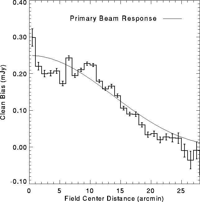
Figure: Bias in the peak flux density as a function of the distance of a source from field center in the CLEANed grid images, derived from artificial sources inserted in the data and comparisons of sources observed in overlapping grid images. The bias is the value that must be added to the peak flux density to get the correct flux. The shape of the primary beam response is also shown; because the bias is essentially identical in shape to the beam, the bias in coadded images is uniform across the field.

This correction is made simpler by the radial dependence of the CLEAN bias. When the individual grid images are corrected for the primary beam response to create the coadded images, the radial dependence disappears; consequently the bias in the coadded images of  mJy/beam ([BWH95]) is independent of source position.

Unfortunately, the magnitude of the bias also depends on the image RMS and can be twice as large in very noisy images. High RMS fields are most often the result of the presence of a very bright source (S > 1 Jy) whose sidelobes are not adequately removed from the image. Similar problems are associated with very extended sources which are also CLEANed incompletely. The distribution of grid image RMS values, shown in Figure 3, demonstrates that significant CLEAN bias underestimates are rare. Only 2% of our 11,000 grid images have RMS values as much as 30% higher than the median RMS. These problematic sky positions can be readily identified from the survey coverage map.

  
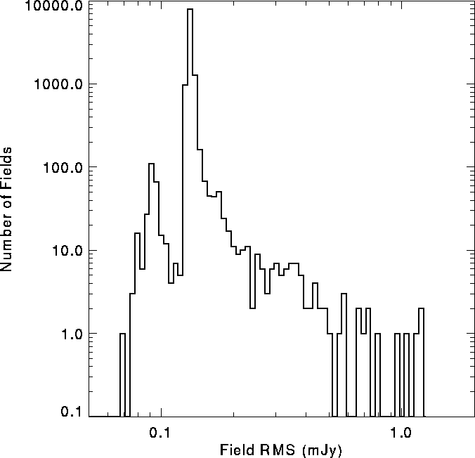
Figure: Histogram of the RMS noise in grid images. The vast majority of fields have RMS values  mJy/beam. The secondary peak around 0.09 mJy/beam is due to fields that were observed twice. Fields containing very bright sources account for the tail at higher RMS values.

The catalog format

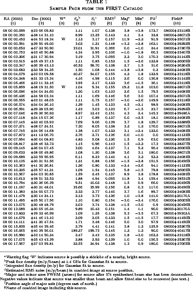
Table 1 is a sample from the on-line FIRST catalog. The column entries are as follows:

1,2:

The right ascension and declination of the source (J2000); position errors are dependent on source size and extent (see § 5.4).

3:

A `W' in this column is a warning flag that the source may be a sidelobe of a nearby bright source (see § 4.2).

4,5:

The peak and integrated flux densities ( , , quoted in mJy/beam and mJy respectively) derived from the elliptical Gaussian fits (§ 3) and corrected for CLEAN bias (§ 4.3).

6:

The local noise rms estimate ( , mJy/beam) derived as described in § 2. Note that the source detection significance is , not , because of the CLEAN bias correction to the peak flux density.

7-9:

The major and minor axes (FWHM in arcseconds) and the position angle (degrees east of north) of the fitted Gaussian with the synthesized beam size subtracted in quadrature. Noise can cause the fitted values of the axes before deconvolution to be smaller than the beam; to preserve this information in the catalog, the listed sizes are negative when the fitted size is smaller than the beam. When the deconvolved size quoted in the catalog , the fitted size was ; when , . For most purposes, the best estimate of the true source size is either the listed size or zero, whichever is greater.

10:

The field name of the coadded image from which the catalog entry was derived (note that a given source may also be found in other images); the field name encodes the position of the field center as hhmmm+ddmmm where RA = hh mm.m and Dec = dd mm.m. Field names ending with an `A' were constructed entirely from 1993 observations, while those with a `B' include at least some data from the 1994 session. This nomenclature will be extended in the obvious way in the years to come, with `C' referring to data from 1995, etc. This suffix provides a rough indication of the epoch of the observation, although some `B' fields do contain data from both 1993 and 1994.

The catalog from the coadded images obtained in 1993 was released in preliminary form (95jan06 version) through our WWW page (http://sundog.stsci.edu). The release described herein (95oct16 version) includes 138,665 sources from an area of 1550  .